All the data originates in analog signals from a BBQ system installed in the LHC tunnel.
The analog signals, for both, the horizontal (H) and vertical (V) planes, were converted into two streams of integer numbers using 24-bit analog-to-digital converters (ADCs).
Each LHC revolution lasting about 90 microseconds there was produced one number corresponding to the actual beam position in each of the two machine planes for each of the two LHC beams.
All these numbers were stored in the logging database and later were used to produce presented here sound records and plots.
At the same time numbers were processed by a front-end computer located close to the LHC tunnel, to produce beam signal spectra, which could be displayed in the control room and used in the tune feedback system.
The tune feedback system uses tune readings from the BBQ systems and calculates in real time currents for the quadrupole corrector magnets so that the magnetic filed they produce results in the desired betatron tunes of both LHC beams.
Below are links to sound .wav records, which were produced from the BBQ signal samples.
The sampling rate of the records corresponds exactly to the rate at which the original analog signals were sampled (that is the LHC revolution frequency of 11 245 Hz), so the listened sound is as you would be listening to the original BBQ analog signals.
In the first file the left (L) stereo channel contains a record of beam oscillations in the horizontal plane and the right (R) stereo channel a record of beam oscillations in the vertical plane.
In the second file both stereo channels contain only the record of the horizontal beam oscillations.
In the third file both stereo channels contain only the record of the vertical beam oscillations.
In the fourth special file both stereo channels contain first 1 s of H injection oscillations and then 1 s of V injection oscillations.
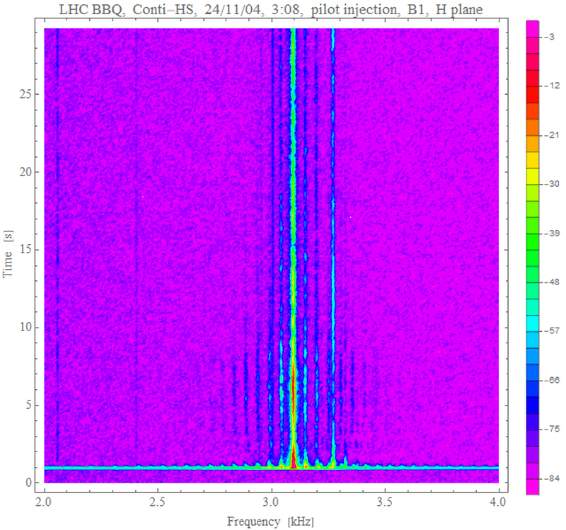
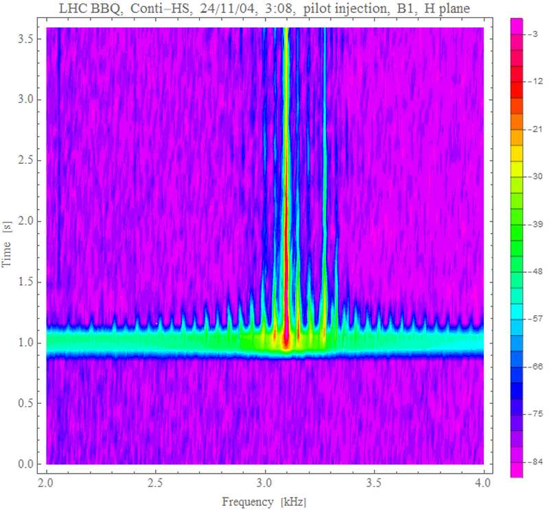
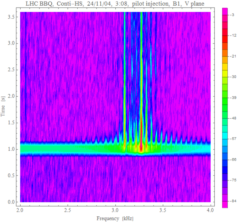
This way you can hear well the frequency difference between the H tune frequency of about 3.1 kHz and the V tune frequency of about 3.3 kHz.
Headphones help a lot to resolve different components !
- H+V : both planes, H in L channel, V in R channel
- H : only H plane in both stereo channels
- V : only V plane In both stereo channels
- H and then V : in both stereo channels, first 1 s of H, then 1 s of V
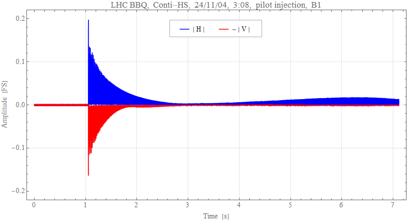
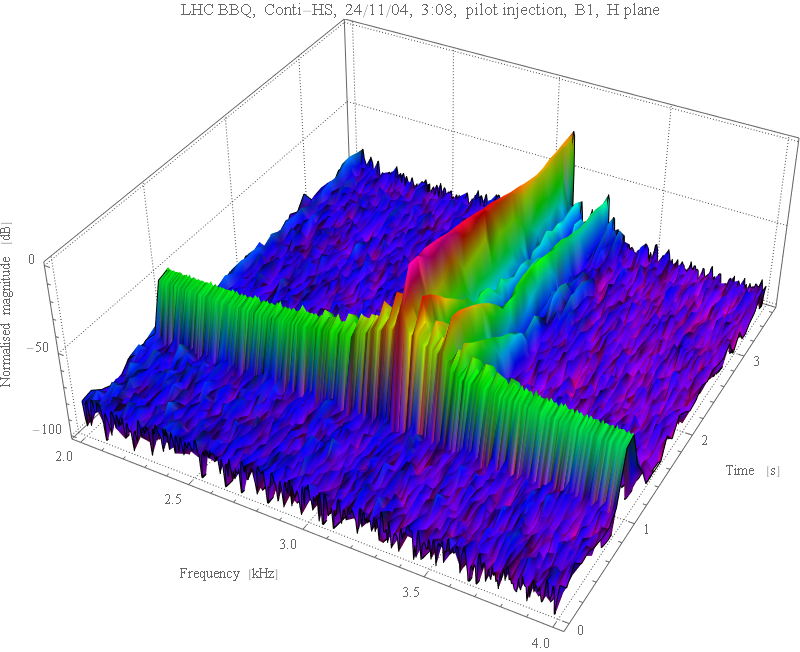
Below are shown plots of the H and V BBQ signal waveforms.
As beam oscillation signals are symmetric, the plots show their absolute values (envelopes).
For the left linear scale plot the vertical plane envelope is inverted to be plotted below the time axis, so that signals from both H and V planes can be presented on one plot.
The right plot has logarithmic amplitude axis to deal with the large dynamic range of the BBQ signals.
In both plots the signals are normalised to the full dynamic range of the system (FS = Full Scale).

Fig. 1a. Envelopes of the H and V beam oscillation amplitudes.

Fig. 1b. Envelopes of the H and V beam oscillation amplitudes in the logarithmic scale.