Marek GASIOR - Home page

Home >> Professional >> 3D-BBQ >> LHC Results >> Last two physics beam injections

Presented BBQ data produced by the Continuous High-Sensitivity system was automatically logged on 4/11/24 (fill #10312), when last two physics beam injections went into LHC ring 1, the penultimate around 3:38.

Please note:

Spectra in both planes are dominated by mains harmonics.

Measuring tunes on so busy spectra is very difficult if not impossible, so in such conditions gated BBQ systems often perform better, despite their lower sensitivity.
In gated systems only a few bunches are measured, for which the transverse damper gain is smaller and whose oscillations are therefore less reduced.

Corresponding data acquired with the Continuous Gated system is presented in Example 5b .

Below are links to sound .wav records, which were produced from the BBQ signal samples.
The sampling rate of the records corresponds exactly to the rate at which the original analog signals were sampled (that is the LHC revolution frequency of 11 245 Hz), so the listened sound is as you would be listening to the original BBQ analog signals.

In the first file the left (L) stereo channel contains a record of beam oscillations in the horizontal (H) plane and the right (R) stereo channel a record of beam oscillations in the vertical plane (V).
In the second file both stereo channels contain only the record of the horizontal beam oscillations.
In the third file both stereo channels contain only the record of the vertical beam oscillations.

H+V : both planes, H in L channel, V in R channel
H : only H plane in both stereo channels
V : only V plane In both stereo channels

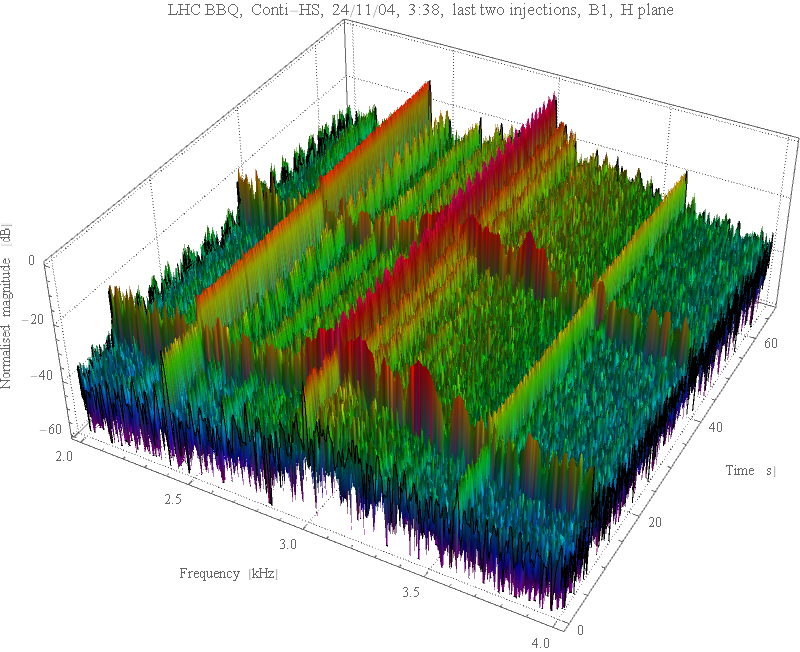
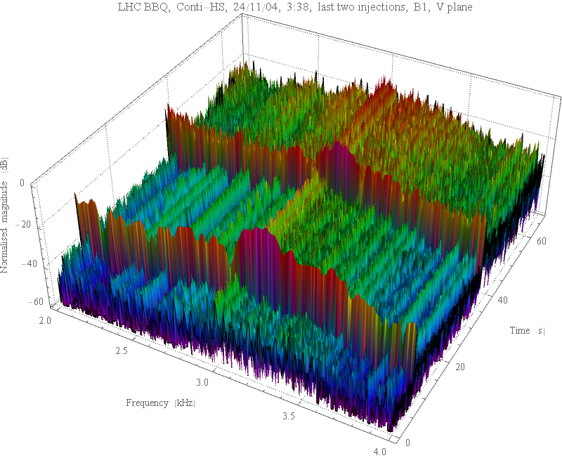
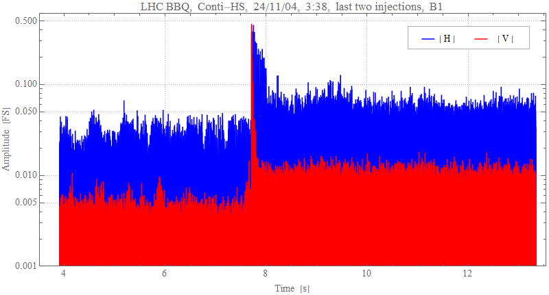
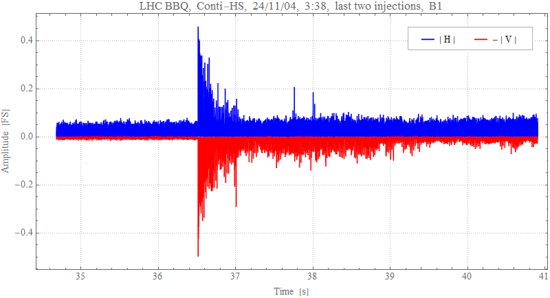
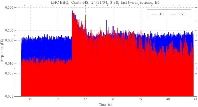
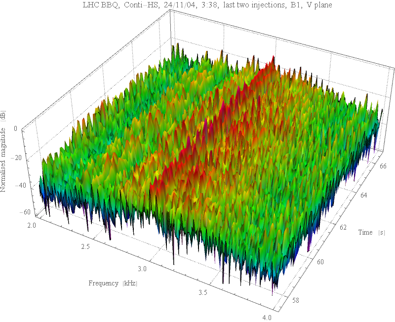
Below are shown plots of the H and V BBQ signal envelopes in linear and logarithmic scales.

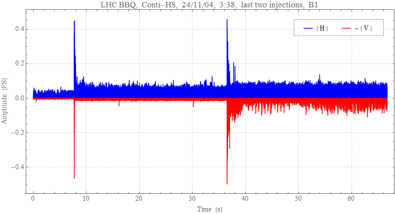
Fig. 1a. Envelopes of the H and V beam oscillation amplitudes.

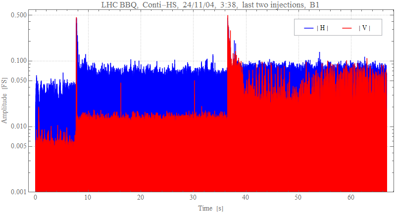
Fig. 1b. Envelopes of the H and V beam oscillation amplitudes in the logarithmic scale.

H and V signal records were divided into segments lasting 0.2 s (so each segment has 0.2 * 11 245 samples), with 0.1 s (50 %) overlap, so there are 10 such segments per second.
Samples of each segment were multiplied by the Hann window, prior to calculating their Discrete Fourier Transform (DFT) to obtain discrete magnitude spectra, whose frequency resolution is 1/(0.2 s) = 5 Hz.
As there are 10 signal segments in the time domain, there are also 10 spectra per second.

Magnitude spectra of H (left) and V (right) signals calculated this way are shown below for frequencies in the range 2 - 4 kHz, where most interesting beam motion components are located.
The spectrum magnitude is normalised to the strongest spectral component in the whole record and expressed in decibels, to reveal the large dynamic range of the beam spectral content.

Fig. 2h. H plane magnitude spectra.

Fig. 2v. V plane magnitude spectra.

The figures below show contour plots corresponding to the spectra in the above Fig. 2h and 2v.

Fig. 3h. Contour plot corresponding to the H magnitude spectra of Fig. 2h

Fig. 3v. Contour plot corresponding to the V magnitude spectra of Fig. 2v

The figures below show plots of the magnitude spectra at selected characteristic times, listed in the plots.

Fig. 4h. H spectra at the times listed in the plots.
The spectra correspond to cross-sections of the above 3D and contour plots.

Fig. 4v. V spectra at the times listed in the plots.
The spectra correspond to cross-sections of the above 3D and contour plots.

Below are shown plots zoomed to the time around the penultimate injection, based on exactly the same processing as the plots above.

Fig. 5a. Envelopes of the H and V beam oscillation amplitudes.

Fig. 5b. Envelopes of the H and V beam oscillation amplitudes in the logarithmic scale.

The magnitude spectra shown below are normalised to the strongest spectral component in the whole record and expressed in decibels, to reveal the large dynamic range of the beam spectral content.

Fig. 6h. H plane magnitude spectra.

Fig. 6v. V plane magnitude spectra.

The figures below show contour plots corresponding to the spectra in the above Fig. 6h and 6v.

Fig. 7h. Contour plot corresponding to the H magnitude spectra of Fig. 6h

Fig. 7v. Contour plot corresponding to the V magnitude spectra of Fig. 6v

Below are shown plots zoomed to the time around the last injection, based on exactly the same processing as the plots above.